
Deep Dream是谷歌公司在2015年公布的一项有趣的技术。在训练好的卷积神经网络中,只需要设定几个参数,就可以通过这项技术生成一张图像。
本文章的代码和图片都放在我的github上,想实现本文代码的同学建议大家可以先把代码Download下来,再参考本文的解释,理解起来会更加方便。
疑问:
- 卷积层究竟学习到了什么内容?
- 卷积层的参数代表的意义是什么?
- 浅层的卷积和深层的卷积学习到的内容有哪些区别?
设输入网络的图形为x,网络输出的各个类别的概率为$t$(1000维的向量,代表了1000种类别的概率),我们以t[100]的某一类别为优化目标,不断地让神经网络去调整输入图像x的像素值,让输出t[100]尽可能的大,最后得到下图图像。
极大化某一类概率得到的图片
卷积的一个通道就可以代表一种学习到的“信息” 。以某一个通道的平均值作为优化目标,就可以弄清楚这个通道究竟学习到了什么,这也是Deep Dream 的基本原理。在下面的的小节中, 会以程序的形式,更详细地介绍如何生成并优化Deep Dream 图像。
TensorFlow中的Deep Dream模型
导入Inception模型
原始的Deep Dream模型只需要优化ImageNet模型卷积层某个通道的激活值就可以了,为此,应该先在TensorFlow导入一个ImageNet图像识别模型。这里以Inception模型为例进行介绍,对应程序的文件名为load_inception.py。
以下是真正导入Inception模型。TensorFlow为提供了一种特殊的以“.pb”为扩展名的文件,可以事先将模型导入到pb文件中,再在需要的时候导出。对于Inception模型,对应的pb文件为tensorflow_inception_graph.pb。
# 创建图和Session
graph = tf.Graph()
sess = tf.InteractiveSession(graph=graph)

# tensorflow_inception_graph.pb文件中,既存储了inception的网络结构也存储了对应的数据
# 使用下面的语句将之导入
model_fn = 'tensorflow_inception_graph.pb'
with tf.gfile.FastGFile(model_fn, 'rb') as f:
    graph_def = tf.GraphDef()
    graph_def.ParseFromString(f.read())
# 定义t_input为我们输入的图像
t_input = tf.placeholder(tf.float32, name='input')
imagenet_mean = 117.0       # 图片像素值的 均值
# 输入图像需要经过处理才能送入网络中
# expand_dims是加一维,从[height, width, channel]变成[1, height, width, channel]
# 因为Inception模型输入格式是(batch, height, width,channel)。
t_preprocessed = tf.expand_dims(t_input - imagenet_mean, 0)
# 将数据导入模型
tf.import_graph_def(graph_def, {'input': t_preprocessed})
导入模型后,找出模型中所有的卷积层,并尝试输出某个卷积层的形状:
# 找到所有卷积层
layers = [op.name for op in graph.get_operations()
            if op.type == 'Conv2D' and 'import/' in op.name]

# 输出卷积层层数
print('Number of layers', len(layers))  # Number of layers 59

# 特别地,输出mixed4d_3x3_bottleneck_pre_relu的形状
name = 'mixed4d_3x3_bottleneck_pre_relu'
print('shape of %s: %s' %
      (name, str(graph.get_tensor_by_name('import/' + name + ':0').get_shape())))
# shape of mixed4d_3x3_bottleneck_pre_relu: (?, ?, ?, 144)
# 因为不清楚输入图像的个数以及大小,所以前三维的值是不确定的,显示为问号
生成原始的Deep Dream图像
我们定义一个保存图像的函数,以便我们把模型输出的数据保存为图像。
def savearray(img_array, img_name):
    """把numpy.ndarray保存图片"""
    scipy.misc.toimage(img_array).save(img_name)
    print('img saved: %s' % img_name)
输入图像,生成某一通道图像
# 定义卷积层、通道数,并取出对应的tensor
name = 'mixed4d_3x3_bottleneck_pre_relu'
layer_output = graph.get_tensor_by_name("import/%s:0" % name)   # 该层输出为(? , ?, ? , 144)
# 因此channel可以取0~143中的任何一个整数值
channel = 139
# 定义原始的图像噪声 作为初始的图像优化起点
img_noise = np.random.uniform(size=(224, 224, 3)) + 100.0
# 调用render_naive函数渲染
render_naive(layer_output[:, :, :, channel], img_noise, iter_n=20)
计算梯度,不断迭代渲染初始图片
def render_naive(t_obj, img0, iter_n=20, step=1.0):
    """通过调整输入图像t_input,来让优化目标t_score尽可能的大
    :param t_obj: 卷积层某个通道的值
    :param img0:初始化噪声图像
    :param iter_n:迭代数
    :param step:学习率
    """
    # t_score是优化目标。它是t_obj的平均值
    # t_score越大,就说明神经网络卷积层对应通道的平均激活越大
    t_score = tf.reduce_mean(t_obj)
    # 计算t_score对t_input的梯度
    t_grad = tf.gradients(t_score, t_input)[0]

    # 创建新图
    img = img0.copy()
    for i in range(iter_n):
        # 在sess中计算梯度,以及当前的score
        g, score = sess.run([t_grad, t_score], {t_input: img})
        # 对img应用梯度。step可以看做“学习率”
        g /= g.std() + 1e-8
        img += g * step
        print('score(mean)=%f' % score)
    # 保存图片
    savearray(img, 'naive.jpg')
经过20次迭代后,会把图像保存为naive.jpg,
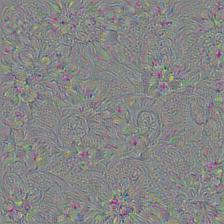
确实可以通过最大化某一通道的平均值得到一些有意义的图像!此处图像的生成效果还不太好,
生产更大尺寸的Deep Dream图像
首先尝试生成更大尺寸的图像,在上面生成图像的尺寸是(224, 224, 3),这正是传递的img_noise的大小。如果传递更大的img_noise,就可以生成更大的图片。
产生问题:会占用更大的内存(或显存),若想生成特别大的图片,就会因为内存不足而导致渲染失败。
解决办法:把图片分成几个部分,每次只对图片的一个部分做优化,这样每次优化时只会消耗固定大小的内存。
def calc_grad_tiled(img, t_grad, tile_size=512):
    """可以对任意大小的图像计算梯度
    :param img: 初始化噪声图片
    :param t_grad: 优化目标(score)对输入图片的梯度
    :param tile_size: 每次只对tile_size×tile_size大小的图像计算梯度,避免内存问题
    :return: 返回梯度更新后的图像
    """
    sz = tile_size  # 512
    h, w = img.shape[:2]
    # 防止在tile的边缘产生边缘效应对图片进行整体移动
    # 产生两个(0,sz]之间均匀分布的整数值
    sx, sy = np.random.randint(sz, size=2)
    # 先在水平方向滚动sx个位置,再在垂直方向上滚动sy个位置
    img_shift = np.roll(np.roll(img, sx, 1), sy, 0)
    grad = np.zeros_like(img)
    # x, y是开始位置的像素
    for y in range(0, max(h - sz // 2, sz), sz):  # 垂直方向
        for x in range(0, max(w - sz // 2, sz), sz):  # 水平方向
            # 每次对sub计算梯度。sub的大小是tile_size×tile_size
            sub = img_shift[y:y + sz, x:x + sz]
            g = sess.run(t_grad, {t_input: sub})
            grad[y:y + sz, x:x + sz] = g
    # 使用np.roll滚动回去
    return np.roll(np.roll(grad, -sx, 1), -sy, 0)
在实际工程中,为了加快图像的收敛速度,采用先生成小尺寸,再将图片放大的方法
def resize_ratio(img, ratio):
    """将图片img放大ratio倍"""
    min = img.min()  # 图片的最小值
    max = img.max()  # 图片的最大值
    img = (img - min) / (max - min) * 255  # 归一化
    # 把输出缩放为0~255之间的数
    print("魔", img.shape)
    img = np.float32(scipy.misc.imresize(img, ratio))
    print("鬼", img.shape)
    img = img / 255 * (max - min) + min  # 将像素值缩放回去
    return img


def render_multiscale(t_obj, img0, iter_n=10, step=1.0, octave_n=3, octave_scale=1.4):
    """生成更大尺寸的图像
    :param t_obj:卷积层某个通道的值
    :param img0:初始化噪声图像
    :param iter_n:迭代数
    :param step:学习率
    :param octave_n: 放大一共会进行octave_n-1次
    :param octave_scale: 图片放大倍数,大于1的"浮点数"则会变成原来的倍数!整数会变成百分比
    :return:
    """
    # 同样定义目标和梯度
    t_score = tf.reduce_mean(t_obj)  # 定义优化目标
    t_grad = tf.gradients(t_score, t_input)[0]  # 计算t_score对t_input的梯度

    img = img0.copy()
    print("原始尺寸",img.shape)
    for octave in range(octave_n):
        if octave > 0:
            # 将小图片放大octave_scale倍
            # 共放大octave_n - 1 次
            print("前", img.shape)
            img = resize_ratio(img, octave_scale)
            print("后", img.shape)
        for i in range(iter_n):
            # 调用calc_grad_tiled计算任意大小图像的梯度
            g = calc_grad_tiled(img, t_grad)    # 对图像计算梯度
            g /= g.std() + 1e-8
            img += g * step
    savearray(img, 'multiscale.jpg')
octave_n越大,最后生成的图像就会越大,默认的octave_n=3。有了上面的代码,直接调用函数即可实现
if __name__ == '__main__':
    name = 'mixed4d_3x3_bottleneck_pre_relu'
    channel = 139
    img_noise = np.random.uniform(size=(224, 224, 3)) + 100.0
    layer_output = graph.get_tensor_by_name("import/%s:0" % name)
    render_multiscale(layer_output[:, :, :, channel], img_noise, iter_n=20)
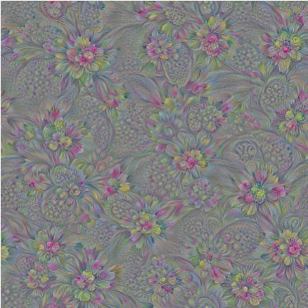
此时可以看到,卷积层“mixed4d_3x3_bottleneck_pre_rel”的第139个通道实际上就是学习到了某种花朵的特征,如果输入这种花朵的图像,它的激活值就会达到最大。大家还可以调整octave_n为更大的值,就可以生成更大的图像。不管最终图像的尺寸是多大,始终只会对512 * 512像素的图像计算梯度,因此内存始终是够用的。如果在读者的环境中,计算512 * 512的图像的梯度会造成内存问题,可以将函数中tile_size修改为更小的值。
生成更高质量的Deep Dream图像
我们将关注点转移到“质量”上,上一节生成的图像在细节部分变化还比较剧烈,而希望图像整体的风格应该比较“柔和”。
在图像处理算法中,有高频成分和低频成分的概念:
- 高频成分:图像中灰度、颜色、明度变化比较剧烈的地方,如边缘、细节部分
- 低频成分:图像变化不大的地方,如大块色块、整体风格
上图生成的高频成分太多,而我们希望图像的低频成分应该多一些,这样生成的图像才会更加“柔和”。
解决方法:
- 对高频成分加入损失。这样图像在生成的时候就因为新加入损失的作用而发生改变。但加入损失会导致计算量和收敛步数的增加。
- 放大低频的梯度。之前生成图像时,使用的梯度是统一的。如果可以对梯度作分解,将之分为“高频梯度”“低频梯度”,再人为地去放大“低频梯度”,就可以得到较为柔和的图像了。
拉普拉斯金字塔(LaplacianPyramid)对图像进行分解。这种算法可以把图片分解为多层,底层的level1、level2对应图像的高频成分,上层的level3、level4对应图像的低频成分。

我们可以对梯度也做拉普拉斯金字塔分解。分解之后,对高频的梯度和低频的梯度都做标准化,可以让梯度的低频成分和高频成分差不多,表现在图像上就会增加图像的低频成分,从而提高生成图像的质量。通常称这种方法为拉普拉斯金字塔梯度标准化(Laplacian Pyramid GradientNormalization)。
下面是拉普拉斯金字塔梯度标准化实现的代码,代码我已经详细注释,实现流程
- 首先将原始图片分解成n-1个高频成分,和1个低频成分
- 然后对每层都进行标准化
- 将标准化后的高频成分和低频成分相加
k = np.float32([1, 4, 6, 4, 1])
k = np.outer(k, k)  # 计算两个向量的外积(5, 5)
k5x5 = k[:, :, None, None] / k.sum() * np.eye(3, dtype=np.float32)  # (5, 5, 3, 3)


# 这个函数将图像分为低频成分和高频成分
def lap_split(img):
    with tf.name_scope('split'):
        # 做过一次卷积相当于一次“平滑”,因此lo为低频成分
        # filter=k5x5=[filter_height, filter_width, in_channels, out_channels]
        lo = tf.nn.conv2d(img, k5x5, [1, 2, 2, 1], 'SAME')
        # 低频成分放缩到原始图像一样大小
        # value,filter,output_shape,strides
        lo2 = tf.nn.conv2d_transpose(lo, k5x5 * 4, tf.shape(img), [1, 2, 2, 1])
        # 用原始图像img减去lo2,就得到高频成分hi
        hi = img - lo2
    return lo, hi


# 这个函数将图像img分成n层拉普拉斯金字塔
def lap_split_n(img, n):
    levels = []
    for i in range(n):
        # 调用lap_split将图像分为低频和高频部分
        # 高频部分保存到levels中
        # 低频部分再继续分解
        img, hi = lap_split(img)
        levels.append(hi)
    levels.append(img)
    return levels[::-1]  # 倒序,把低频放在最前面


# 将拉普拉斯金字塔还原到原始图像
def lap_merge(levels):
    img = levels[0]  # 低频
    for hi in levels[1:]:  # 高频
        with tf.name_scope('merge'):
            # value,filter,output_shape,strides
            # 卷积后变成低频,转置卷积将低频还原成图片的高频
            img = tf.nn.conv2d_transpose(img, k5x5 * 4, tf.shape(hi), [1, 2, 2, 1]) + hi
    return img


# 对img做标准化。
def normalize_std(img, eps=1e-10):
    with tf.name_scope('normalize'):
        std = tf.sqrt(tf.reduce_mean(tf.square(img)))
        # 返回的是a, b之间的最大值
        return img / tf.maximum(std, eps)


# 拉普拉斯金字塔标准化
def lap_normalize(img, scale_n=4):
    img = tf.expand_dims(img, 0)
    # 将图片分解成拉普拉斯金字塔
    tlevels = lap_split_n(img, scale_n)
    # 每一层都做一次normalize_std
    tlevels = list(map(normalize_std, tlevels))
    # 将拉普拉斯金字塔还原到原始图像
    out = lap_merge(tlevels)
    return out[0, :, :, :]
函数解释:
- lap_split函数:可以把图像分解为高频成分和低频成分。其中对原始图像做一次卷积就得到低频成分lo。这里的卷积起到的作用就是“平滑”,以提取到图片中变化不大的部分。得到低频成分后,使用转置卷积将低频成分缩放到原图一样的大小lo2,再用原图img减去lo2就可以得到高频成分了。
- lap_split_n函数:它将图像分成n层的拉普拉斯金字塔,每次都调用lap_split对当前图像进行分解,分解得到的高频成分就保存到金字塔levels中,而低频成分则留待下一次分解。
- lap_merge函数:将一个分解好的拉普拉斯金字塔还原成原始图像,
- normalize_std函数:对图像进行标准化。
- lap_normalize函数:就是将输入图像分解为拉普拉斯金字塔,然后调用normalize_std对每一层进行标准化,输出为融合后的结果。
有了拉普拉斯金字塔标准化的函数后,就可以写出生成图像的代码:
def tffunc(*argtypes):
    # 将一个对Tensor定义的函数转换成一个正常的对numpy.ndarray定义的函数
    placeholders = list(map(tf.placeholder, argtypes))

    def wrap(f):
        out = f(*placeholders)

        def wrapper(*args, **kw):
            return out.eval(dict(zip(placeholders, args)), session=kw.get('session'))

        return wrapper

    return wrap


def render_lapnorm(t_obj, img0, iter_n=10, step=1.0, octave_n=3, octave_scale=1.4, lap_n=4):
    """
    :param t_obj: 目标分数,某一通道的输出值 layer_output[:,:,:,channel] (?, ?, ?, 144)
    :param img0: 输入图片,噪声图像 size=(224, 224, 3)
    :param iter_n: 迭代次数
    :param step: 学习率
    """
    t_score = tf.reduce_mean(t_obj)     # 定义优化目标
    t_grad = tf.gradients(t_score, t_input)[0]  # 定义梯度
    # 将lap_normalize转换为正常函数,partial:冻结函数一个参数
    lap_norm_func = tffunc(np.float32)(partial(lap_normalize, scale_n=lap_n))

    img = img0.copy()
    for octave in range(octave_n):
        if octave > 0:
            img = resize_ratio(img, octave_scale)
        for i in range(iter_n):
            # 计算图像梯度
            g = calc_grad_tiled(img, t_grad)
            # 唯一的区别在于我们使用lap_norm_func来标准化g!
            g = lap_norm_func(g)  # 对梯度,进行了拉普拉斯变换
            img += g * step
            print('.', end=' ')
    savearray(img, 'lapnorm.jpg')
tffunc函数,它的功能是将一个对Tensor定义的函数转换成一个正常的对numpy.ndarray定义的函数。上面定义的lap_normalize的输入参数是一个Tensor,而输出也是一个Tensor,利用tffunc函数可以将它变成一个输入ndarray类型,输出也是ndarray类型的函数。
最终生成图像的代码也与之前类似,只需要调用render_lapnorm函数即可:
if __name__ == '__main__':
    name = 'mixed4d_3x3_bottleneck_pre_relu'
    channel = 139
    img_noise = np.random.uniform(size=(224, 224, 3)) + 100.0
    layer_output = graph.get_tensor_by_name("import/%s:0" % name)
    render_lapnorm(layer_output[:, :, :, channel], img_noise, iter_n=20)
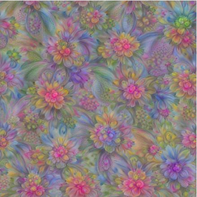
与上节对比,本节确实在一定程度上提高了生成图像的质量。也可以更清楚地看到这个卷积层中的第139个通道学习到的图像特征。大家可以尝试不同的通道。
最终的Deep Dream模型
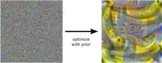
前面我们分别介绍了如何通过极大化卷积层某个通道的平均值来生成图像,并学习了如何生成大尺寸和更高质量的图像。最终的Deep Dream模型还需要对图片添加一个背景。
其实之前是从image_noise开始优化图像的,现在使用一张背景图像作为起点对图像进行优化就可以了。
def resize(img, hw):
    # 参数hw是一个元组(tuple),用(h, w)的形式表示缩放后图像的高和宽。
    min = img.min()
    max = img.max()
    img = (img - min) / (max - min) * 255
    img = np.float32(scipy.misc.imresize(img, hw))
    img = img / 255 * (max - min) + min
    return img

ef render_deepdream(t_obj, img0, iter_n=10, step=1.5, octave_n=4, octave_scale=1.4):
    t_score = tf.reduce_mean(t_obj)
    t_grad = tf.gradients(t_score, t_input)[0]

    img = img0
    # 同样将图像进行金字塔分解
    # 此时提取高频、低频的方法比较简单。直接缩放就可以
    octaves = []
    for i in range(octave_n - 1):
        hw = img.shape[:2]
        # 图片方法生成低频成分 lo
        lo = resize(img, np.int32(np.float32(hw) / octave_scale))
        hi = img - resize(lo, hw)   # 高频成分
        img = lo
        octaves.append(hi)

    # 先生成低频的图像,再依次放大并加上高频
    for octave in range(octave_n):
        # 0 1 2 3
        if octave > 0:
            hi = octaves[-octave]
            img = resize(img, hi.shape[:2]) + hi
        for i in range(iter_n):
            g = calc_grad_tiled(img, t_grad)
            img += g * (step / (np.abs(g).mean() + 1e-7))

    img = img.clip(0, 255)
    savearray(img, 'deepdream1.jpg')

if __name__ == '__main__':
    img0 = PIL.Image.open('test.jpg')
    img0 = np.float32(img0)

    name = 'mixed4d_3x3_bottleneck_pre_relu'
    channel = 139
    layer_output = graph.get_tensor_by_name("import/%s:0" % name)
    render_deepdream(layer_output[:, :, :, channel], img0)
这里改了3个部分,读入图像‘test.jpg',并将它作为起点,传递给函数render_deepdream。为了保证图像生成的质量,render_deepdream对图像也进行高频低频的分解。分解的方法是直接缩小原图像,就得到低频成分lo,其中缩放图像使用的函数是resize,它的参数hw是一个元组(tuple),用(h, w)的形式表示缩放后图像的高和宽。
在生成图像的时候,从低频的图像开始。低频的图像实际上就是缩小后的图像,经过一定次数的迭代后,将它放大再加上原先的高频成分。计算梯度的方法同样使用的是calc_grad_tiled方法。


左图为原始的test.jpg图片,右图为生成的Deep Dream图片
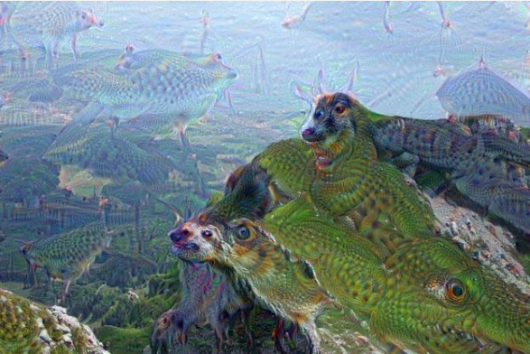
利用下面的代码可以生成非常著名的含有动物的DeepDream图片,此时优化的目标是mixed4c的全体输出。
name = "mixed4c"
layer_optput = graph.get_tensor_by_name("import/%s:0" % name)
render_deepdream(tf.square(layer_optput), img0)
大家可以自行尝试不同的背景图像,不同的通道数,不同的输出层,就可以得到各种各样的生成图像。
参考
文章来源: 博客园
- 还没有人评论,欢迎说说您的想法!


 客服
客服


