Tutorial on Hidden Markov Model

 

Contents

• What's HMM
• Three Central Issues
• Evaluation problem
• Learning problem
• Decoding problem
• Words in the end
• Reference

What's HMM?

    In problems that have an inherent temporality -- that is, consist of a process that unfolds in time -- we may have states at time t that are influenced directly by a state t-1. Hidden Markov model (HMM) have found greatest use in such problem, for instance speech recognition or gesture recongnition.

    HMM has two stochastic process. One is a Markov chain and the other is a "emission" that based on each Markov chain's state.

    The Markov chain can be decribed as Figure 1

Figure 1

    The state space in Markov chain is $mathbf{W}$
[
mathbf{W} = {w_1, w_2, ..., w_n}
]

    The state at time t is $w(t)$ and a particular sequence of length T is denoted by $mathbf{w^T}$.
[
mathbf{w^T} = {w(1), w(2), ..., w(T) }
]

    where $w(t) = w_i$, $i = 1,2,...,n$

    The hidden Markov model can be described as Figure 2.

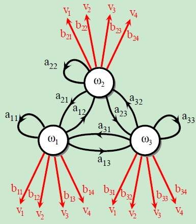
Figure 2

    At every time step t the system is in a state $w(t)$ but now it emits some (visible) symbol $v(t)$. Notice that $v(t)$ can be discrete or continuous, but in the passage, $v(t)$ is assumed to be discrete.

    We define a particular sequence of such visible states as
[mathbf{V^T} = {v(1), v(2), ..., v(T)}]

    where $v(t) = v_i$, $i=1,2,3,...$

    We denote the initial distrubution $pi_i$, transition probabilities $a_{ij}$ among hidden states and for the probability $b_{jk}$ of the emission of a visible state:
[
begin{split}
& pi_i = P(w(1)=w_i) \
& a_{ij}(t) = Pleft(w(t+1)=w_j|w(t)=w_iright)\
& b_{jk}(t) = Pleft(v(t)=v_k|w(t)=w_jright)
end{split}
]

    We have the normalization condition:
[
begin{split}
& sum_{j}a_{ij}(t) = 1\
& sum_{k}b_{jk}(t) = 1
end{split}
]

    Let $mathbf{A}=[a_{ij}]_{ntimes n}$ , $mathbf{B}=[b_{jk}]_{ntimes m}$ and $mathbf{pi} = (pi_i)$, then the HMM can be described as $mathbf{lambda} = (mathbf{A},mathbf{B},mathbf{pi})$

Three Central Issues

    When we get an HMM we need to handle three central issues in order to make full use of HMM　and have a better understanding of HMM.

    ① The Evaluation problem

    Suppose we have an HMM. Determine the probability that a particular sequence of visible states $mathbf{V^T}$ generated by that model.

    ② The Learning problem

Suppose we are given the coarse structure of a model (the number of hidden states and the number of visible states) but not the probability $a_{ij}$, $b_{jk}$ and $pi_i$. Given a set of training observation of visible symbols, determine these parameters.

    ③ The Decoding problem

    Suppose we have an HMM as well as a set of observation $mathbf{V^T}$. Determine the most likely sequence of hidden states $mathbf{w^T}$ that led to those observation.

    We will consider each of these problem in turn.

Evaluation problem

    Evaluation problem: Given $mathbf{lambda} = (mathbf{A},mathbf{B},mathbf{pi})$ and observation sequence $mathbf{V^T}$, compute $P(mathbf{V^T}|mathbf{lambda})$.

    If we compute $P(mathbf{V^T}|mathbf{lambda})$ directly:
[
begin{split}
P(mathbf{V^T}|mathbf{lambda}) &= sum_{mathbf{w^T}}P(mathbf{V^T}|mathbf{w^T},mathbf{lambda})P(mathbf{w^T}|mathbf{lambda})\
& = sum_{mathbf{w^T}}prod_{t=1}^{T}pi_i a_{ij}(t) b_{jk}(t)
end{split}
]

    Analyze the formulation above, $w^T$ totally have $n^T$ situations. Thus, it is an $O(Tn^T)$ calculation, which is quite prohibitive in practice.

    A computationaly simpler algorithm -- forward algorithm and backward algorithm -- for the same goal is as follows. Notice that both forward algorithm and backward algorithm can calculate $P(mathbf{V^T}|mathbf{lambda})$.

Forward algorithm

    Define forward variable:
[
alpha_t(i) = P(V^t,w(t)=w_i|lambda)
]

   Then,
[
begin{split}
alpha_1(i) &= P(v(1)=v_k,w(1)=w_i|lambda) \
& = P(v(1)=v_k|w(1)=w_i,lambda)P(w(1)=w_i|lambda)\
& = pi_i b_{ik}(1)
end{split}
]
[
begin{split}
alpha_{t+1}(j) &= left[ sum_{i=1}^{N}alpha_t(i)a_{ij}(t) right] b_{jk}(t+1)\
1leq &tleq T-1, qquad 1leq jleq n
end{split}
]

[
P(mathbf{V^T}|mathbf{lambda}) = sum_{i=1}^{n}alpha_T(i)
]

Backward algorithm

    Define backward varible:
[
begin{split}
beta_t(i) &= P(V^T/V^t|w(t)=w_i,lambda)\
& = P(v(t+1),v(t+2),...,v(T)|w(t)=w_i,lambda)
end{split}
]

    Then,
[
begin{split}
beta_T(i) = 1
end{split}
]

[
begin{split}
beta_i(t) &= sum_{j=1}^{n}a_{ij}b_{jk}(t+1)beta_j(t+1)\
1leq &tleq T-1, qquad 1leq ileq n
end{split}
]

[
begin{split}
P(mathbf{V^T}|mathbf{lambda}) & = sum_{i=1}^{n}pi_i b_{ik}(1) beta_1(i)\
& = sum_{i=1}^{n}alpha_1(i) beta_1(i)
end{split}
]

    The complexity of both forward and backward algorithm is $O(Tn^2)$, rather than the direct algorithm's complexity $O(Tn^T)$ !

Some probability calculation

    ① Given $lambda$ and observation $V^T$, the probability of $w(t)=w_i$ is :
[
begin{split}
gamma_t(i) & = P(w(t)=w_i|V^T,lambda)\
& = frac{P(w(t)=w_i,V^T|lambda)}{P(V^T|lambda)}\
& = frac{alpha_t(i)beta_t(i)}{P(V^T|lambda)}\
& = frac{alpha_t(i)beta_t(i)}{sum_{i=1}^{n}alpha_t(i)beta_t(i)}
end{split}
]

    ② Given $lambda$ and observation $V^T$, the probability of $w(t)=w_icap w(t+1)=w_j$:
[
begin{split}
xi_t(i,j) &= P(w(t)=w_i,w(t+1)=w_j|V^T,lambda)\
& = frac{P(w(t)=w_i,w(t+1)=w_j,V^T|lambda)}{P(V^T|lambda)}\
& = frac{P(w(t)=w_i,w(t+1)=w_j,V^T|lambda)}{sum_{i=1}^{n}sum_{j=1}^{n}P(w(t)=w_i,w(t+1)=w_j,V^T|lambda)}\
& = frac{alpha_t(i)a_{ij}b_{jk}(t+1)beta_{t+1}(j)}{sum_{i=1}^{n}sum_{j=1}^{n}alpha_t(i)a_{ij}b_{jk}(t+1)beta_{t+1}(j)}
end{split}
]

    ③ We can get some expectation value.

    (1) The expectation value of state i in condition of observation $V^T$:
[
sum_{t=1}^{T}gamma_t(i)
]

    (2) The expectation value of the times that transform from state i to the another state:
[
sum_{t=1}^{T-1}gamma_t(i)
]

    (3) The expectation value of the times that transform from state i to state j:
[
sum_{t=1}^{T-1}xi_t(i,j)
]

Learning problem

    Learning problem : Given the observation $V^T$(obvious variable) without $w^T$(hidden variable), compute the parameters of $lambda = (A,B,pi)$.

    The parameter learining can be completed by EM algorithm(Also called Baum-Welch algorithm).

    The log likehood function of the hidden variable and obvious variable:
[
L = log P(V^T,w^T|lambda)
]

    The Q function can be writen as:
[
begin{split}
Q(lambda,lambda^0) &=sum_{w^T}log P(V^T,w^T|lambda) P(w^T|V^T,lambda^0) \
& = sum_{w^T}log P(V^T,w^T|lambda) frac{P(V^T,w^T|lambda^0)}{P(V^T|lambda^0)}
end{split}
]

    Thus,
[
begin{split}
lambda &= argmaxlimits_{lambda}Q(lambda,lambda^0)\
& = argmaxlimits_{lambda} sum_{w^T}log P(V^T,w^T|lambda) frac{P(V^T,w^T|lambda^0)}{P(V^T|lambda^0)}\
& = argmaxlimits_{lambda} sum_{w^T}log P(V^T,w^T|lambda) P(V^T,w^T|lambda^0)
end{split}
]

    Finnaly, we can get:
[
begin{split}
a_{ij} &= frac{sum_{t=1}^{T-1}xi_t(i,j)}{sum_{t=1}^{T-1}gamma_t(i)}\
b_{jk}(t) &= frac{sum_{t=1,v(t)=v_k}^{T}gamma_t(j)}{sum_{t=1}^{T}gamma_t(j)}\
pi_i & = gamma_1(i)
end{split}
]

    Thus, Baum-Welch algorithm can be described as follows:

    ① Initialize. In terms of n=0, choose $a_{ij}^{(0)}$, $b_{jk}^{(0)}(t)$ and $pi_i^{(0)}$, and get $lambda{(0)}=(A^{(0)},B^{(0)},pi^{(0)})$

    ② Recursion. for n=1,2,...
[
begin{split}
a_{ij}^{(n+1)} &= frac{sum_{t=1}^{T-1}xi_t(i,j)}{sum_{t=1}^{T-1}gamma_t(i)}\
b_{jk}^{(n+1)}(t) &= frac{sum_{t=1,v(t)=v_k}^{T}gamma_t(j)}{sum_{t=1}^{T}gamma_t(j)}\
pi_i^{(n+1)} & = gamma_1(i)
end{split}
]

    ③ If satisfy the termination condition, algorithm done. Otherwise, go to ②.

Decoding problem

    Decoding problem: Given the observation $V^T$ and model parameters $lambda = (A,B,pi)$, calculate the most likely hidden state $w^T$.

To solve decoding problem, we can use Viterbi algorithm, which is a dynamic programming.

    Define variable:
[
delta_t(i) = maxlimits_{w(1),...,w(t-1)}P(w(t)=w_i,w(t-1),...,w(1),v(t),...,v(1)|lambda), qquad i = 1,2,...,n
]

    then,
[
delta_{t+1}(j) = left[maxlimits_{i}delta_t(i)a_{ij}right]b_{jk}(t+1)
]

    Define variable:
[
psi_t(i) = argmaxlimits_{1leq jleq}[delta_{t-1}(j)a_{ji}]
]

    So, Vaterbi algorithm can be described as follows:

    ① Initialization.
[
begin{split}
delta_1(i) &= P(w(1)=w_i,v(1)|lambda)\
& = P(v(1)=v_k|w(1)=w_i)P(w(1)=w_i)\
& = pi_i b_{ik}(1), qquad i=1,2,...,n\
psi_1(i) &= 0, qquad i=1,2,...,n
end{split}
]

    ② Recursion. For t=2,3,...,T
[
begin{split}
delta_{t}(i) &= left[maxlimits_{j}delta_{t-1}(j)a_{ji}right]b_{ik}(t), qquad i=1,2,...,n\
psi_t(i) & = maxlimits_{j}delta_{t-1}(j)a_{ji}, qquad i=1,2,...,n
end{split}
]

    ③ Termination.
[
begin{split}
P^* &= maxlimits_{i}delta_T(i)\
i_T^* & = argmaxlimits_{i}delta_T(i)
end{split}
]

    ④ Backtracking. For t=T-1,...,1
[
i_t^* = psi_{t+1}(i_t+1^*)
]

    Finally, we can get the optimal path $I^*=(i^*_1,i^*_2,...,i^*_T)$

Words in the end

    At the begining of the new term, I complete this eassy eventually. The purpose that I write this $'Hiddenquad Markovquad Model'$ is to have an understanding of HMM and practice my English writing skill, which is kind of disfluency...I'm sorry :( ...

    The are also some quension after I complete this eassy:

    ① The relationship between HMM and PGM(Probabilistic Graphical Model). There are some probability calculation in forward algorithm and backward algorithm and they are quite related to PGM.

    ② In Baum-Welch algorithm, how to use Lagrange method to find the solution?

    ③ In HMM learning problem, how to deal with multiple sequence when trainning the model?

 

Reference

[1] 李航.统计学习方法[M].北京:清华大学出版社.

[2] LAWRENCE R. RABINER.A Tutorial on Hidden Markov Models and
Selected Applications in Speech Recognition[J].PROCEEDINGS OF THE IEEE,FEBRUARY 1989

[3] 刘成林.中国科学院大学《模式识别》PPT

• 还没有人评论，欢迎说说您的想法！