
摘要:为了评价模型的泛化能力,即判断模型的好坏,我们需要用某个指标来衡量,有了评价指标,就可以对比不同模型的优劣,并通过这个指标来进一步调参优化模型。
本文分享自华为云社区《目标检测模型的评价指标详解及代码实现》,作者:嵌入式视觉。
前言
为了了解模型的泛化能力,即判断模型的好坏,我们需要用某个指标来衡量,有了评价指标,就可以对比不同模型的优劣,并通过这个指标来进一步调参优化模型。对于分类和回归两类监督模型,分别有各自的评判标准。
不同的问题和不同的数据集都会有不同的模型评价指标,比如分类问题,数据集类别平衡的情况下可以使用准确率作为评价指标,但是现实中的数据集几乎都是类别不平衡的,所以一般都是采用 AP 作为分类的评价指标,分别计算每个类别的 AP,再计算mAP。
一,精确率、召回率与F1
1.1,准确率
准确率(精度) – Accuracy,预测正确的结果占总样本的百分比,定义如下:
准确率=(TP+TN)/(TP+TN+FP+FN)
错误率和精度虽然常用,但是并不能满足所有任务需求。以西瓜问题为例,假设瓜农拉来一车西瓜,我们用训练好的模型对西瓜进行判别,现如精度只能衡量有多少比例的西瓜被我们判断类别正确(两类:好瓜、坏瓜)。但是若我们更加关心的是“挑出的西瓜中有多少比例是好瓜”,或者”所有好瓜中有多少比例被挑出来“,那么精度和错误率这个指标显然是不够用的。
虽然准确率可以判断总的正确率,但是在样本不平衡的情况下,并不能作为很好的指标来衡量结果。举个简单的例子,比如在一个总样本中,正样本占 90%,负样本占 10%,样本是严重不平衡的。对于这种情况,我们只需要将全部样本预测为正样本即可得到 90% 的高准确率,但实际上我们并没有很用心的分类,只是随便无脑一分而已。这就说明了:由于样本不平衡的问题,导致了得到的高准确率结果含有很大的水分。即如果样本不平衡,准确率就会失效。
1.2,精确率、召回率
精确率(查准率)P、召回率(查全率)R 的计算涉及到混淆矩阵的定义,混淆矩阵表格如下:
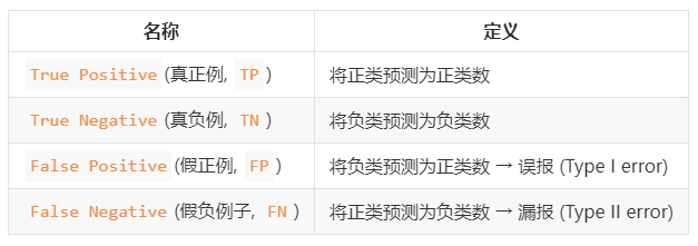
查准率与查全率计算公式:
- 查准率(精确率)P=TP/(TP+FP)P=TP/(TP+FP)
- 查全率(召回率)R=TP/(TP+FN)R=TP/(TP+FN)
精准率和准确率看上去有些类似,但是完全不同的两个概念。精准率代表对正样本结果中的预测准确程度,而准确率则代表整体的预测准确程度,既包括正样本,也包括负样本。
精确率描述了模型有多准,即在预测为正例的结果中,有多少是真正例;召回率则描述了模型有多全,即在为真的样本中,有多少被我们的模型预测为正例。精确率和召回率的区别在于分母不同,一个分母是预测为正的样本数,另一个是原来样本中所有的正样本数。
1.3,F1 分数
如果想要找到 P 和 R 二者之间的一个平衡点,我们就需要一个新的指标:F1 分数。F1 分数同时考虑了查准率和查全率,让二者同时达到最高,取一个平衡。F1 计算公式如下:
这里的 F1 计算是针对二分类模型,多分类任务的 F1 的计算请看下面。

F1 度量的一般形式:Fβ,能让我们表达出对查准率/查全率的偏见,Fβ 计算公式如下:

其中β>1 对查全率有更大影响,β<1 对查准率有更大影响。
不同的计算机视觉问题,对两类错误有不同的偏好,常常在某一类错误不多于一定阈值的情况下,努力减少另一类错误。在目标检测中,mAP(mean Average Precision)作为一个统一的指标将这两种错误兼顾考虑。
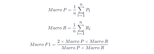
很多时候我们会有多个混淆矩阵,例如进行多次训练/测试,每次都能得到一个混淆矩阵;或者是在多个数据集上进行训练/测试,希望估计算法的”全局“性能;又或者是执行多分类任务,每两两类别的组合都对应一个混淆矩阵;…总而来说,我们希望能在 nn 个二分类混淆矩阵上综合考虑查准率和查全率。
一种直接的做法是先在各混淆矩阵上分别计算出查准率和查全率,记为 (P1,R1),(P2,R2),...,(Pn,Rn) 然后取平均,这样得到的是”宏查准率(Macro-P)“、”宏查准率(Macro-R)“及对应的”宏 F1F1(Macro-F1)“:
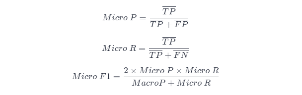
另一种做法是将各混淆矩阵对应元素进行平均,得到 TP、FP、TN、FNTP、FP、TN、FN 的平均值,再基于这些平均值计算出”微查准率“(Micro-P)、”微查全率“(Micro-R)和”微 F1“(Mairo-F1)
1.4,PR 曲线
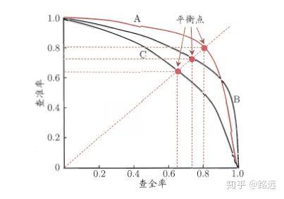
精准率和召回率的关系可以用一个 P-R 图来展示,以查准率 P 为纵轴、查全率 R 为横轴作图,就得到了查准率-查全率曲线,简称 P-R 曲线,PR 曲线下的面积定义为 AP:
1.4.1,如何理解 P-R 曲线
可以从排序型模型或者分类模型理解。以逻辑回归举例,逻辑回归的输出是一个 0 到 1 之间的概率数字,因此,如果我们想要根据这个概率判断用户好坏的话,我们就必须定义一个阈值 。通常来讲,逻辑回归的概率越大说明越接近 1,也就可以说他是坏用户的可能性更大。比如,我们定义了阈值为 0.5,即概率小于 0.5 的我们都认为是好用户,而大于 0.5 都认为是坏用户。因此,对于阈值为 0.5 的情况下,我们可以得到相应的一对查准率和查全率。
但问题是:这个阈值是我们随便定义的,我们并不知道这个阈值是否符合我们的要求。 因此,为了找到一个最合适的阈值满足我们的要求,我们就必须遍历 0 到 1 之间所有的阈值,而每个阈值下都对应着一对查准率和查全率,从而我们就得到了 PR 曲线。
最后如何找到最好的阈值点呢? 首先,需要说明的是我们对于这两个指标的要求:我们希望查准率和查全率同时都非常高。 但实际上这两个指标是一对矛盾体,无法做到双高。图中明显看到,如果其中一个非常高,另一个肯定会非常低。选取合适的阈值点要根据实际需求,比如我们想要高的查全率,那么我们就会牺牲一些查准率,在保证查全率最高的情况下,查准率也不那么低。。
1.5,ROC 曲线与 AUC 面积
- PR 曲线是以 Recall 为横轴,Precision 为纵轴;而 ROC 曲线则是以 FPR 为横轴,TPR 为纵轴**。P-R 曲线越靠近右上角性能越好。PR 曲线的两个指标都聚焦于正例
- PR 曲线展示的是 Precision vs Recall 的曲线,ROC 曲线展示的是 FPR(x 轴:False positive rate) vs TPR(True positive rate, TPR)曲线。
- [ ] ROC 曲线
- [ ] AUC 面积
二,AP 与 mAP
2.1,AP 与 mAP 指标理解
AP 衡量的是训练好的模型在每个类别上的好坏,mAP 衡量的是模型在所有类别上的好坏,得到 AP 后 mAP 的计算就变得很简单了,就是取所有 AP 的平均值。AP 的计算公式比较复杂(所以单独作一章节内容),详细内容参考下文。
mAP 这个术语有不同的定义。此度量指标通常用于信息检索、图像分类和目标检测领域。然而这两个领域计算 mAP 的方式却不相同。这里我们只谈论目标检测中的 mAP 计算方法。
mAP 常作为目标检测算法的评价指标,具体来说就是,对于每张图片检测模型会输出多个预测框(远超真实框的个数),我们使用 IoU (Intersection Over Union,交并比)来标记预测框是否预测准确。标记完成后,随着预测框的增多,查全率 R 总会上升,在不同查全率 R 水平下对准确率 P 做平均,即得到 AP,最后再对所有类别按其所占比例做平均,即得到 mAP 指标。
2.2,近似计算AP

知道了AP 的定义,下一步就是理解AP计算的实现,理论上可以通过积分来计算AP,公式如下:

但通常情况下都是使用近似或者插值的方法来计算 AP。

- 近似计算 AP (approximated average precision),这种计算方式是 approximated 形式的;
- 很显然位于一条竖直线上的点对计算 AP 没有贡献;
- 这里 N 为数据总量,k 为每个样本点的索引, Δr(k)=r(k)−r(k−1)。
近似计算 AP 和绘制 PR 曲线代码如下:
import numpy as np
import matplotlib.pyplot as plt
class_names = ["car", "pedestrians", "bicycle"]
def draw_PR_curve(predict_scores, eval_labels, name, cls_idx=1):
 """calculate AP and draw PR curve, there are 3 types
    Parameters:
    @all_scores: single test dataset predict scores array, (-1, 3)
    @all_labels: single test dataset predict label array, (-1, 3)
    @cls_idx: the serial number of the AP to be calculated, example: 0,1,2,3...
    """
 # print('sklearn Macro-F1-Score:', f1_score(predict_scores, eval_labels, average='macro'))
 global class_names
    fig, ax = plt.subplots(nrows=1, ncols=1, figsize=(15, 10))
 # Rank the predicted scores from large to small, extract their corresponding index(index number), and generate an array
 idx = predict_scores[:, cls_idx].argsort()[::-1]
 eval_labels_descend = eval_labels[idx]
 pos_gt_num = np.sum(eval_labels == cls_idx) # number of all gt
 predict_results = np.ones_like(eval_labels)
 tp_arr = np.logical_and(predict_results == cls_idx, eval_labels_descend == cls_idx) # ndarray
 fp_arr = np.logical_and(predict_results == cls_idx, eval_labels_descend != cls_idx)
 tp_cum = np.cumsum(tp_arr).astype(float) # ndarray, Cumulative sum of array elements.
 fp_cum = np.cumsum(fp_arr).astype(float)
 precision_arr = tp_cum / (tp_cum + fp_cum) # ndarray
 recall_arr = tp_cum / pos_gt_num
    ap = 0.0
 prev_recall = 0
 for p, r in zip(precision_arr, recall_arr):
      ap += p * (r - prev_recall)
 # pdb.set_trace()
 prev_recall = r
 print("------%s, ap: %f-----" % (name, ap))
 fig_label = '[%s, %s] ap=%f' % (name, class_names[cls_idx], ap)
 ax.plot(recall_arr, precision_arr, label=fig_label)
 ax.legend(loc="lower left")
 ax.set_title("PR curve about class: %s" % (class_names[cls_idx]))
 ax.set(xticks=np.arange(0., 1, 0.05), yticks=np.arange(0., 1, 0.05))
 ax.set(xlabel="recall", ylabel="precision", xlim=[0, 1], ylim=[0, 1])
 fig.savefig("./pr-curve-%s.png" % class_names[cls_idx])
 plt.close(fig)
2.3,插值计算 AP
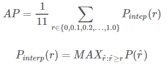
插值计算(Interpolated average precision) APAP 的公式的演变过程这里不做讨论,详情可以参考这篇文章,我这里的公式和图也是参考此文章的。11 点插值计算方式计算 APAP 公式如下:

- 这是通常意义上的 11 points_Interpolated 形式的 AP,选取固定的 0,0.1,0.2,…,1.00,0.1,0.2,…,1.0 11 个阈值,这个在 PASCAL2007 中使用
- 这里因为参与计算的只有 11 个点,所以 K=11,称为 11 points_Interpolated,k 为阈值索引
- Pinterp(k) 取第 k 个阈值所对应的样本点之后的样本中的最大值,只不过这里的阈值被限定在了 0,0.1,0.2,…,1.00,0.1,0.2,…,1.0 范围内。

从曲线上看,真实 AP< approximated AP < Interpolated AP,11-points Interpolated AP 可能大也可能小,当数据量很多的时候会接近于 Interpolated AP,与 Interpolated AP 不同,前面的公式中计算 AP 时都是对 PR 曲线的面积估计,PASCAL 的论文里给出的公式就更加简单粗暴了,直接计算11 个阈值处的 precision 的平均值。PASCAL 论文给出的 11 点计算 AP 的公式如下。
1、在给定 recal 和 precision 的条件下计算 AP:
def voc_ap(rec, prec, use_07_metric=False):
 """
    ap = voc_ap(rec, prec, [use_07_metric])
    Compute VOC AP given precision and recall.
    If use_07_metric is true, uses the
    VOC 07 11 point method (default:False).
    """
 if use_07_metric:
 # 11 point metric
        ap = 0.
 for t in np.arange(0., 1.1, 0.1):
 if np.sum(rec >= t) == 0:
                p = 0
 else:
                p = np.max(prec[rec >= t])
            ap = ap + p / 11.
 else:
 # correct AP calculation
 # first append sentinel values at the end
 mrec = np.concatenate(([0.], rec, [1.]))
 mpre = np.concatenate(([0.], prec, [0.]))
 # compute the precision envelope
 for i in range(mpre.size - 1, 0, -1):
 mpre[i - 1] = np.maximum(mpre[i - 1], mpre[i])
 # to calculate area under PR curve, look for points
 # where X axis (recall) changes value
 i = np.where(mrec[1:] != mrec[:-1])[0]
 # and sum (Delta recall) * prec
        ap = np.sum((mrec[i + 1] - mrec[i]) * mpre[i + 1])
 return ap
2、给定目标检测结果文件和测试集标签文件 xml 等计算 AP:
def parse_rec(filename):
 """ Parse a PASCAL VOC xml file
 Return : list, element is dict.
    """
    tree = ET.parse(filename)
    objects = []
 for obj in tree.findall('object'):
 obj_struct = {}
 obj_struct['name'] = obj.find('name').text
 obj_struct['pose'] = obj.find('pose').text
 obj_struct['truncated'] = int(obj.find('truncated').text)
 obj_struct['difficult'] = int(obj.find('difficult').text)
 bbox = obj.find('bndbox')
 obj_struct['bbox'] = [int(bbox.find('xmin').text),
 int(bbox.find('ymin').text),
 int(bbox.find('xmax').text),
 int(bbox.find('ymax').text)]
 objects.append(obj_struct)
 return objects
def voc_eval(detpath,
 annopath,
 imagesetfile,
 classname,
 cachedir,
 ovthresh=0.5,
             use_07_metric=False):
 """rec, prec, ap = voc_eval(detpath,
 annopath,
 imagesetfile,
 classname,
                                [ovthresh],
                                [use_07_metric])
    Top level function that does the PASCAL VOC evaluation.
 detpath: Path to detections result file
 detpath.format(classname) should produce the detection results file.
 annopath: Path to annotations file
 annopath.format(imagename) should be the xml annotations file.
 imagesetfile: Text file containing the list of images, one image per line.
 classname: Category name (duh)
 cachedir: Directory for caching the annotations
    [ovthresh]: Overlap threshold (default = 0.5)
    [use_07_metric]: Whether to use VOC07's 11 point AP computation
        (default False)
    """
 # assumes detections are in detpath.format(classname)
 # assumes annotations are in annopath.format(imagename)
 # assumes imagesetfile is a text file with each line an image name
 # cachedir caches the annotations in a pickle file
 # first load gt
 if not os.path.isdir(cachedir):
 os.mkdir(cachedir)
 cachefile = os.path.join(cachedir, '%s_annots.pkl' % imagesetfile)
 # read list of images
 with open(imagesetfile, 'r') as f:
        lines = f.readlines()
 imagenames = [x.strip() for x in lines]
 if not os.path.isfile(cachefile):
 # load annotations
        recs = {}
 for i, imagename in enumerate(imagenames):
            recs[imagename] = parse_rec(annopath.format(imagename))
 if i % 100 == 0:
 print('Reading annotation for {:d}/{:d}'.format(
 i + 1, len(imagenames)))
 # save
 print('Saving cached annotations to {:s}'.format(cachefile))
 with open(cachefile, 'wb') as f:
 pickle.dump(recs, f)
 else:
 # load
 with open(cachefile, 'rb') as f:
 try:
                recs = pickle.load(f)
 except:
                recs = pickle.load(f, encoding='bytes')
 # extract gt objects for this class
 class_recs = {}
 npos = 0
 for imagename in imagenames:
        R = [obj for obj in recs[imagename] if obj['name'] == classname]
 bbox = np.array([x['bbox'] for x in R])
        difficult = np.array([x['difficult'] for x in R]).astype(np.bool)
        det = [False] * len(R)
 npos = npos + sum(~difficult)
 class_recs[imagename] = {'bbox': bbox,
 'difficult': difficult,
 'det': det}
 # read dets
 detfile = detpath.format(classname)
 with open(detfile, 'r') as f:
        lines = f.readlines()
 splitlines = [x.strip().split(' ') for x in lines]
 image_ids = [x[0] for x in splitlines]
    confidence = np.array([float(x[1]) for x in splitlines])
    BB = np.array([[float(z) for z in x[2:]] for x in splitlines])
 nd = len(image_ids)
 tp = np.zeros(nd)
 fp = np.zeros(nd)
 if BB.shape[0] > 0:
 # sort by confidence
 sorted_ind = np.argsort(-confidence)
 sorted_scores = np.sort(-confidence)
        BB = BB[sorted_ind, :]
 image_ids = [image_ids[x] for x in sorted_ind]
 # go down dets and mark TPs and FPs
 for d in range(nd):
            R = class_recs[image_ids[d]]
            bb = BB[d, :].astype(float)
 ovmax = -np.inf
            BBGT = R['bbox'].astype(float)
 if BBGT.size > 0:
 # compute overlaps
 # intersection
 ixmin = np.maximum(BBGT[:, 0], bb[0])
 iymin = np.maximum(BBGT[:, 1], bb[1])
 ixmax = np.minimum(BBGT[:, 2], bb[2])
 iymax = np.minimum(BBGT[:, 3], bb[3])
 iw = np.maximum(ixmax - ixmin + 1., 0.)
 ih = np.maximum(iymax - iymin + 1., 0.)
                inters = iw * ih
 # union
 uni = ((bb[2] - bb[0] + 1.) * (bb[3] - bb[1] + 1.) +
 (BBGT[:, 2] - BBGT[:, 0] + 1.) *
 (BBGT[:, 3] - BBGT[:, 1] + 1.) - inters)
                overlaps = inters / uni
 ovmax = np.max(overlaps)
 jmax = np.argmax(overlaps)
 if ovmax > ovthresh:
 if not R['difficult'][jmax]:
 if not R['det'][jmax]:
 tp[d] = 1.
                        R['det'][jmax] = 1
 else:
 fp[d] = 1.
 else:
 fp[d] = 1.
 # compute precision recall
 fp = np.cumsum(fp)
 tp = np.cumsum(tp)
    rec = tp / float(npos)
 # avoid divide by zero in case the first detection matches a difficult
 # ground truth
 prec = tp / np.maximum(tp + fp, np.finfo(np.float64).eps)
    ap = voc_ap(rec, prec, use_07_metric)
 return rec, prec, ap
2.4,mAP 计算方法
因为 mAP 值的计算是对数据集中所有类别的 AP 值求平均,所以我们要计算 mAP,首先得知道某一类别的 AP 值怎么求。不同数据集的某类别的 AP 计算方法大同小异,主要分为三种:
(1)在 VOC2007,只需要选取当 Recall>=0,0.1,0.2,...,1Recall>=0,0.1,0.2,...,1 共 11 个点时的 Precision 最大值,然后 APAP 就是这 11 个 Precision 的平均值,mAPmAP 就是所有类别 APAP 值的平均。VOC 数据集中计算 APAP 的代码(用的是插值计算方法,代码出自py-faster-rcnn仓库)
(2)在 VOC2010 及以后,需要针对每一个不同的 Recall 值(包括 0 和 1),选取其大于等于这些 Recall 值时的 Precision 最大值,然后计算 PR 曲线下面积作为 AP 值,mAPmAP 就是所有类别 AP 值的平均。
(3)COCO 数据集,设定多个 IOU 阈值(0.5-0.95, 0.05 为步长),在每一个 IOU 阈值下都有某一类别的 AP 值,然后求不同 IOU 阈值下的 AP 平均,就是所求的最终的某类别的 AP 值。
三,目标检测度量标准汇总


四,参考资料
- 目标检测评价标准-AP mAP
- 目标检测的性能评价指标
- Soft-NMS
- Recent Advances in Deep Learning for Object Detection
- A Simple and Fast Implementation of Faster R-CNN
- 分类模型评估指标——准确率、精准率、召回率、F1、ROC曲线、AUC曲线
- 一文让你彻底理解准确率,精准率,召回率,真正率,假正率,ROC/AUC
文章来源: 博客园
- 还没有人评论,欢迎说说您的想法!
 客服
客服


