
前言
边界框:在⽬标检测⾥,我们通常使⽤边界框(bounding box,缩写是 bbox)来描述⽬标位置。边界框是⼀个矩形框,可以由矩形左上⻆的 x 和 y 轴坐标与右下⻆的 x 和 y 轴坐标确定。
检测网络中的一些术语解释:
backbone:翻译为主干网络,主要指用来做特征提取作用的网络,早期分类网络VGG、ResNet等去掉用于分类的全连接层的部分就是backbone网络。neck: 指放在backbone和head之间的网络,作用是更好的融合/利用backbone提取的feature,可以理解为特征增强模块,典型的neck是如FPN结构。head:检测头,输出想要结果(分类+定位)的网络,放在模型最后。如YOLO使用特定维度的conv获取目标的类别和bbox信息。
一,anchor box
⽬标检测算法通常会在输⼊图像中采样⼤量的区域,然后判断这些区域中是否包含我们感兴趣的⽬标,并调整区域边缘从而更准确地预测⽬标的真实边界框(ground-truth bounding box)。不同的模型使⽤的区域采样⽅法可能不同。两阶段检测模型常用的⼀种⽅法是:以每个像素为中⼼⽣成多个⼤小和宽⾼⽐(aspect ratio)不同的边界框。这些边界框被称为锚框(anchor box)。
在 Faster RCNN 模型中,每个像素都生成 9 个大小和宽高比都不同的 anchors。在代码中,anchors 是一组由 generate_anchors.py 生成的矩形框列表。其中每行的 4 个值 (x1,y1,x2,y2) 表示矩形左上和右下角点坐标。9 个矩形共有 3 种形状,长宽比为大约为 {1:1, 1:2, 2:1} 三种, 实际上通过 anchors 就引入了检测中常用到的多尺度方法。generate_anchors.py 的代码如下:
注意,这里生成的只是
base anchors,其中一个 框的左上角坐标为 (0,0) 坐标(特征图左上角)的9个 anchor,后续还需网格化(meshgrid)生成其他anchor。同一个 scale,但是不同的 anchor ratios 生成的 anchors 面积理论上是要一样的。
import numpy as np
import six
from six import __init__  # 兼容python2和python3模块


def generate_anchor_base(base_size=16, ratios=[0.5, 1, 2],
                         anchor_scales=[8, 16, 32]):
    """Generate base anchors by enumerating aspect ratio and scales.

    Args:
        base_size (number): The width and the height of the reference window.
        ratios (list of floats): anchor 的宽高比
        anchor_scales (list of numbers): anchor 的尺度

    Returns: Base anchors in a single-level feature maps.`(R, 4)`.
        bounding box is `(x_{min}, y_{min}, x_{max}, y_{max})`
    """
    import numpy as np
    py = base_size / 2.
    px = base_size / 2.

    anchor_base = np.zeros((len(ratios) * len(anchor_scales), 4),
                           dtype=np.float32)
    for i in six.moves.range(len(ratios)):
        for j in six.moves.range(len(anchor_scales)):
            // 乘以感受野值,得到缩放后的 anchor 大小
            h = base_size * anchor_scales[j] * np.sqrt(ratios[i])
            w = base_size * anchor_scales[j] * np.sqrt(1. / ratios[i])

            index = i * len(anchor_scales) + j
            anchor_base[index, 0] = px - w / 2.
            anchor_base[index, 1] = py - h / 2.

            anchor_base[index, 2] = px + h / 2.
            anchor_base[index, 3] = py + w / 2.
    return anchor_base


# test
if __name__ == "__main__":
    bbox_list = generate_anchor_base()
    print(bbox_list)
程序运行输出如下:
[[ -82.50967 -37.254833 53.254833 98.50967 ]
[-173.01933 -82.50967 98.50967 189.01933 ]
[-354.03867 -173.01933 189.01933 370.03867 ]
[ -56. -56. 72. 72. ]
[-120. -120. 136. 136. ]
[-248. -248. 264. 264. ]
[ -37.254833 -82.50967 98.50967 53.254833]
[ -82.50967 -173.01933 189.01933 98.50967 ]
[-173.01933 -354.03867 370.03867 189.01933 ]]
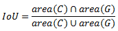
二,IOU
交并比(Intersection-over-Union,IoU),目标检测中使用的一个概念,是模型产生的候选框(candidate bound)与原标记框(ground truth bound)的交叠率,即它们的交集与并集的比值。最理想情况是完全重叠,即比值为 1。计算公式如下:
代码实现如下:
# _*_ coding:utf-8 _*_
# 计算iou

"""
bbox的数据结构为(xmin,ymin,xmax,ymax)--(x1,y1,x2,y2),
每个bounding box的左上角和右下角的坐标
输入:
    bbox1, bbox2: Single numpy bounding box, Shape: [4]
输出:
    iou值
"""
import numpy as np
import cv2

def iou(bbox1, bbox2):
    """
    计算两个bbox(两框的交并比)的iou值
    :param bbox1: (x1,y1,x2,y2), type: ndarray or list
    :param bbox2: (x1,y1,x2,y2), type: ndarray or list
    :return: iou, type float
    """
    if type(bbox1) or type(bbox2) != 'ndarray':
        bbox1 = np.array(bbox1)
        bbox2 = np.array(bbox2)

    assert bbox1.size == 4 and bbox2.size == 4, "bounding box coordinate size must be 4"
    xx1 = np.max((bbox1[0], bbox2[0]))
    yy1 = np.min((bbox1[1], bbox2[1]))
    xx2 = np.max((bbox1[2], bbox2[2]))
    yy2 = np.min((bbox1[3], bbox2[3]))
    bwidth = xx2 - xx1
    bheight = yy2 - yy1
    area = bwidth * bheight  # 求两个矩形框的交集
    union = (bbox1[2] - bbox1[0])*(bbox1[3] - bbox1[1]) + (bbox2[2] - bbox2[0])*(bbox2[3] - bbox2[1]) - area  # 求两个矩形框的并集
    iou = area / union

    return iou


if __name__=='__main__':
    rect1 = (461, 97, 599, 237)
    # (top, left, bottom, right)
    rect2 = (522, 127, 702, 257)
    iou_ret = round(iou(rect1, rect2), 3) # 保留3位小数
    print(iou_ret)

    # Create a black image
    img=np.zeros((720,720,3), np.uint8)
    cv2.namedWindow('iou_rectangle')
    """
    cv2.rectangle 的 pt1 和 pt2 参数分别代表矩形的左上角和右下角两个点,
    coordinates for the bounding box vertices need to be integers if they are in a tuple,
    and they need to be in the order of (left, top) and (right, bottom).
    Or, equivalently, (xmin, ymin) and (xmax, ymax).
    """
    cv2.rectangle(img,(461, 97),(599, 237),(0,255,0),3)
    cv2.rectangle(img,(522, 127),(702, 257),(0,255,0),3)
    font  = cv2.FONT_HERSHEY_SIMPLEX
    cv2.putText(img, 'IoU is ' + str(iou_ret), (341,400), font, 1,(255,255,255),1)
    cv2.imshow('iou_rectangle', img)
    cv2.waitKey(0)
代码输出结果如下所示:

三,Focal Loss
Focal Loss 是在二分类问题的交叉熵(CE)损失函数的基础上引入的,所以需要先学习下交叉熵损失的定义。
3.1,Cross Entropy
在深度学习中我们常使用交叉熵来作为分类任务中训练数据分布和模型预测结果分布间的代价函数。对于同一个离散型随机变量 (textrm{x}) 有两个单独的概率分布 (P(x)) 和 (Q(x)),其交叉熵定义为:
P 表示真实分布, Q 表示预测分布。
但在实际计算中,我们通常不这样写,因为不直观。在深度学习中,以二分类问题为例,其交叉熵损失(CE)函数如下:
其中 (p) 表示当预测样本等于 (1) 的概率,则 (1-p) 表示样本等于 (0) 的预测概率。因为是二分类,所以样本标签 (y) 取值为 ({1,0}),上式可缩写至如下:
为了方便,用 (p_t) 代表 (p),(p_t) 定义如下:
则((3))式可写成:
前面的交叉熵损失计算都是针对单个样本的,对于所有样本,二分类的交叉熵损失计算如下:
其中 (m) 为正样本个数,(n) 为负样本个数,(N) 为样本总数,(m+n=N)。当样本类别不平衡时,损失函数 (L) 的分布也会发生倾斜,如 (m ll n) 时,负样本的损失会在总损失占主导地位。又因为损失函数的倾斜,模型训练过程中也会倾向于样本多的类别,造成模型对少样本类别的性能较差。
再衍生以下,对于所有样本,多分类的交叉熵损失计算如下:
其中,(M) 表示类别数量,(y_{ic}) 是符号函数,如果样本 (i) 的真实类别等于 (c) 取值 1,否则取值 0; (p_{ic}) 表示样本 (i) 预测为类别 (c) 的概率。
对于多分类问题,交叉熵损失一般会结合 softmax 激活一起实现,PyTorch 代码如下,代码出自这里。
import numpy as np

# 交叉熵损失
class CrossEntropyLoss():
    """
    对最后一层的神经元输出计算交叉熵损失
    """
    def __init__(self):
        self.X = None
        self.labels = None

    def __call__(self, X, labels):
        """
        参数:
            X: 模型最后fc层输出
            labels: one hot标注,shape=(batch_size, num_class)
        """
        self.X = X
        self.labels = labels

        return self.forward(self.X)

    def forward(self, X):
        """
        计算交叉熵损失
        参数:
            X:最后一层神经元输出,shape=(batch_size, C)
            label:数据onr-hot标注,shape=(batch_size, C)
        return:
            交叉熵loss
        """
        self.softmax_x = self.softmax(X)
        log_softmax = self.log_softmax(self.softmax_x)
        cross_entropy_loss = np.sum(-(self.labels * log_softmax), axis=1).mean()
        return cross_entropy_loss

    def backward(self):
        grad_x =  (self.softmax_x - self.labels)  # 返回的梯度需要除以batch_size
        return grad_x / self.X.shape[0]

    def log_softmax(self, softmax_x):
        """
        参数:
            softmax_x, 在经过softmax处理过的X
        return:
            log_softmax处理后的结果shape = (m, C)
        """
        return np.log(softmax_x + 1e-5)

    def softmax(self, X):
        """
        根据输入,返回softmax
        代码利用softmax函数的性质: softmax(x) = softmax(x + c)
        """
        batch_size = X.shape[0]
        # axis=1 表示在二维数组中沿着横轴进行取最大值的操作
        max_value = X.max(axis=1)
        #每一行减去自己本行最大的数字,防止取指数后出现inf,性质:softmax(x) = softmax(x + c)
        # 一定要新定义变量,不要用-=,否则会改变输入X。因为在调用计算损失时,多次用到了softmax,input不能改变
        tmp = X - max_value.reshape(batch_size, 1)
        # 对每个数取指数
        exp_input = np.exp(tmp)  # shape=(m, n)
        # 求出每一行的和
        exp_sum = exp_input.sum(axis=1, keepdims=True)  # shape=(m, 1)
        return exp_input / exp_sum
3.2,Balanced Cross Entropy
对于正负样本不平衡的问题,较为普遍的做法是引入 (alpha in(0,1)) 参数来解决,上面公式重写如下:
对于所有样本,二分类的平衡交叉熵损失函数如下:
其中 (frac{alpha}{1-alpha} = frac{n}{m}),即 (alpha) 参数的值是根据正负样本分布比例来决定的,
3.3,Focal Loss Definition
虽然 (alpha) 参数平衡了正负样本(positive/negative examples),但是它并不能区分难易样本(easy/hard examples),而实际上,目标检测中大量的候选目标都是易分样本。这些样本的损失很低,但是由于难易样本数量极不平衡,易分样本的数量相对来讲太多,最终主导了总的损失。而本文的作者认为,易分样本(即,置信度高的样本)对模型的提升效果非常小,模型应该主要关注与那些难分样本(这个假设是有问题的,是 GHM 的主要改进对象)
Focal Loss 作者建议在交叉熵损失函数上加上一个调整因子(modulating factor)((1-p_t)^gamma),把高置信度 (p)(易分样本)样本的损失降低一些。Focal Loss 定义如下:
Focal Loss 有两个性质:
- 当样本被错误分类且 (p_t) 值较小时,调制因子接近于
1,loss几乎不受影响;当 (p_t) 接近于1,调质因子(factor)也接近于0,容易分类样本的损失被减少了权重,整体而言,相当于增加了分类不准确样本在损失函数中的权重。 - (gamma) 参数平滑地调整容易样本的权重下降率,当 (gamma = 0) 时,
Focal Loss等同于CE Loss。 (gamma) 在增加,调制因子的作用也就增加,实验证明 (gamma = 2) 时,模型效果最好。
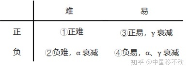
直观地说,调制因子减少了简单样本的损失贡献,并扩大了样本获得低损失的范围。例如,当(gamma = 2) 时,与 (CE) 相比,分类为 (p_t = 0.9) 的样本的损耗将降低 100 倍,而当 (p_t = 0.968) 时,其损耗将降低 1000 倍。这反过来又增加了错误分类样本的重要性(对于 (pt≤0.5) 和 (gamma = 2),其损失最多减少 4 倍)。在训练过程关注对象的排序为正难 > 负难 > 正易 > 负易。
在实践中,我们常采用带 (alpha) 的 Focal Loss:
作者在实验中采用这种形式,发现它比非 (alpha) 平衡形式(non-(alpha)-balanced)的精确度稍有提高。实验表明 (gamma) 取 2,(alpha) 取 0.25 的时候效果最佳。
网上有各种版本的 Focal Loss 实现代码,大多都是基于某个深度学习框架实现的,如 Pytorch和 TensorFlow,我选取了一个较为清晰的代码作为参考,代码来自 这里。
后续有必要自己实现以下,有时间还要去看看
Caffe的实现。
# -*- coding: utf-8 -*-
# @Author  : LG
from torch import nn
import torch
from torch.nn import functional as F

class focal_loss(nn.Module):
    def __init__(self, alpha=0.25, gamma=2, num_classes = 3, size_average=True):
        """
        focal_loss损失函数, -α(1-yi)**γ *ce_loss(xi,yi)
        步骤详细的实现了 focal_loss损失函数.
        :param alpha:   阿尔法α,类别权重.      当α是列表时,为各类别权重,当α为常数时,类别权重为[α, 1-α, 1-α, ....],常用于 目标检测算法中抑制背景类 , retainnet中设置为0.25
        :param gamma:   伽马γ,难易样本调节参数. retainnet中设置为2
        :param num_classes:     类别数量
        :param size_average:    损失计算方式,默认取均值
        """
        super(focal_loss,self).__init__()
        self.size_average = size_average
        if isinstance(alpha,list):
            assert len(alpha)==num_classes   # α可以以list方式输入,size:[num_classes] 用于对不同类别精细地赋予权重
            print(" --- Focal_loss alpha = {}, 将对每一类权重进行精细化赋值 --- ".format(alpha))
            self.alpha = torch.Tensor(alpha)
        else:
            assert alpha<1   #如果α为一个常数,则降低第一类的影响,在目标检测中为第一类
            print(" --- Focal_loss alpha = {} ,将对背景类进行衰减,请在目标检测任务中使用 --- ".format(alpha))
            self.alpha = torch.zeros(num_classes)
            self.alpha[0] += alpha
            self.alpha[1:] += (1-alpha) # α 最终为 [ α, 1-α, 1-α, 1-α, 1-α, ...] size:[num_classes]

        self.gamma = gamma

    def forward(self, preds, labels):
        """
        focal_loss损失计算
        :param preds:   预测类别. size:[B,N,C] or [B,C]    分别对应与检测与分类任务, B 批次, N检测框数, C类别数
        :param labels:  实际类别. size:[B,N] or [B],为 one-hot 编码格式
        :return:
        """
        # assert preds.dim()==2 and labels.dim()==1
        preds = preds.view(-1,preds.size(-1))
        self.alpha = self.alpha.to(preds.device)
        preds_logsoft = F.log_softmax(preds, dim=1) # log_softmax
        preds_softmax = torch.exp(preds_logsoft)    # softmax

        preds_softmax = preds_softmax.gather(1,labels.view(-1,1))
        preds_logsoft = preds_logsoft.gather(1,labels.view(-1,1))
        self.alpha = self.alpha.gather(0,labels.view(-1))
        loss = -torch.mul(torch.pow((1-preds_softmax), self.gamma), preds_logsoft)  # torch.pow((1-preds_softmax), self.gamma) 为focal loss中 (1-pt)**γ

        loss = torch.mul(self.alpha, loss.t())
        if self.size_average:
            loss = loss.mean()
        else:
            loss = loss.sum()
        return loss
mmdetection 框架给出的 focal loss 代码如下(有所删减):
# This method is only for debugging
def py_sigmoid_focal_loss(pred,
                          target,
                          weight=None,
                          gamma=2.0,
                          alpha=0.25,
                          reduction='mean',
                          avg_factor=None):
    """PyTorch version of `Focal Loss <https://arxiv.org/abs/1708.02002>`_.
    Args:
        pred (torch.Tensor): The prediction with shape (N, C), C is the
            number of classes
        target (torch.Tensor): The learning label of the prediction.
        weight (torch.Tensor, optional): Sample-wise loss weight.
        gamma (float, optional): The gamma for calculating the modulating
            factor. Defaults to 2.0.
        alpha (float, optional): A balanced form for Focal Loss.
            Defaults to 0.25.
        reduction (str, optional): The method used to reduce the loss into
            a scalar. Defaults to 'mean'.
        avg_factor (int, optional): Average factor that is used to average
            the loss. Defaults to None.
    """
    pred_sigmoid = pred.sigmoid()
    target = target.type_as(pred)
    pt = (1 - pred_sigmoid) * target + pred_sigmoid * (1 - target)
    focal_weight = (alpha * target + (1 - alpha) *
                    (1 - target)) * pt.pow(gamma)
    loss = F.binary_cross_entropy_with_logits(
        pred, target, reduction='none') * focal_weigh
    return loss
四,NMS
4.1,NMS 介绍
在目标检测中,常会利用非极大值抑制算法(NMS,non maximum suppression)对生成的大量候选框进行后处理,去除冗余的候选框,得到最佳检测框(bbox),以加快目标检测的效,其本质思想搜素局部最大值,抑制非极大值。许多目标检测模型都利用到了 NMS 算法,如 DPM,YOLO,SSD,Faster R-CNN 等。NMS过程如下图所示:
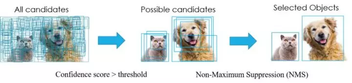
以上图为例,每个选出来的 Bounding Box 检测框(即 BBox)用(x,y,h,w, confidence score,Pdog,Pcat)表示,confidence score 表示 background 和 foreground 的置信度得分,取值范围[0,1]。Pdog, Pcat 分布代表类别是狗和猫的概率。如果是 100 类的目标检测模型,BBox 输出向量为 5+100=105。
4.2,NMS 算法过程
NMS 的目的就是除掉重复的边界框,其主要是通过迭代的形式,不断地以最大得分的框去与其他框做 IoU 操作,并过滤那些 IoU 较大的框。
其实现的思想主要是将各个框的置信度进行排序,然后选择其中置信度最高的框 A,将其作为标准选择其他框,同时设置一个阈值,当其他框 B 与 A 的重合程度超过阈值就将 B 舍弃掉,然后在剩余的框中选择置信度最大的框,重复上述操作。多目标检测的 NMS 算法过程如下:
for object in all objects:
1. 将所有 bboxs 按照 confidence 排序,并标记当前 confidence 最大的 bbox,即要保留的 bbox;
2. 计算当前最大 confidence 对应的 bbox 和剩下所有 bbox 的 IOU;
3. 去除 IOU 大于设定阈值的 bbox,得到新的 bboxs;
4. 对于新生下来的 bboxs,循环执行步骤 2、3,直到所有的 bbox 都满足要求(即无法再移除 bbox)。
nms 的 python 代码如下:
import numpy as np

def py_nms(bboxs, thresh):
    """Pure Python NMS baseline.注意,这里的计算都是在矩阵层面上计算的
    greedily select boxes with high confidence and overlap with current maximum <= thresh
    rule out overlap >= thresh
    :param bboxs: [[x1, y1, x2, y2 score],] # ndarray, shape(-1,5)
    :param thresh: retain overlap < thresh
    :return: indexes to keep
    """
    if(bboxs) == 0:
        return [][]
    bboxs = npa.array(bboxs)
    # 计算 n 个候选框的面积大小
    x1 = bboxs[:,0]
    x2 = bboxs[:, 1]
    y1 = bboxs[:, 2]
    y2 = bboxs[:, 3]
    scores = bboxs[:, 4]
    areas = (x2 - x1 + 1)*(y2 - y1 + 1)

    # 1,对bboxs 按照置信度排序,获取排序后的下标号,argsort 函数默认从小到大排序
    order = np.argsort(scores)  # order shape is (4,)
    picked_bboxs = []

    while order.size > 0:
        # 1, 保留当前 confidence 最大的 bbox加入到返回框列表中
        index = order[-1]
        picked_bboxs.append(bboxs[index]]

        # 2,计算当前 confidence 最大的 bbox 和剩下 bbox 的 IOU
        xx1 = np.maximum(x1[-1], x1[order[:-1]])
        xx2 = np.maximum(x2[-1], x2[order[:-1]])
        yy1 = np.maximum(y1[-1], y1[order[:-1]])
        yy1 = np.maximum(y2[-1], y2[order[:-1]])

        # 计算相交框的面积,注意矩形框不相交时 w 或 h 算出来会是负数,用0代替
        w = np.maximum(0.0, xx2 - xx1 + 1)
        h = np.maximum(0.0, yy2 - yy1 + 1)
        overlap_area = w * h

        IOUs = overlap_area/(areas[index] + areas[order[:-1]] - overlap_area)

        # 3,只保留 `IOU` 小于设定阈值的 `bbox`,得到新的 `bboxs`,更新剩下来 bbox的索引
        remain_index = np.where(IOUs < thresh)  # np.where 来找到符合条件的 index
        order = order[remain_index]
    return picked_bboxs

# test
if __name__ == "__main__":
    bboxs = np.array([[30, 20, 230, 200, 1],
                     [50, 50, 260, 220, 0.9],
                     [210, 30, 420, 5, 0.8],
                     [430, 280, 460, 360, 0.7]])
    thresh = 0.35
    keep_bboxs = py_nms(bboxs, thresh)
    print(keep_bboxs)
程序输出如下:
[0, 2, 3]
[[ 30. 20. 230. 200. 1. ]
[210. 30. 420. 5. 0.8]
[430. 280. 460. 360. 0.7]]
另一个版本的 nms 的 python 代码如下:
from __future__ import print_function
import numpy as np
import time

def intersect(box_a, box_b):
    max_xy = np.minimum(box_a[:, 2:], box_b[2:])
    min_xy = np.maximum(box_a[:, :2], box_b[:2])
    inter = np.clip((max_xy - min_xy), a_min=0, a_max=np.inf)
    return inter[:, 0] * inter[:, 1]

def get_iou(box_a, box_b):
    """Compute the jaccard overlap of two sets of boxes.  The jaccard overlap
    is simply the intersection over union of two boxes.
    E.g.:
        A ∩ B / A ∪ B = A ∩ B / (area(A) + area(B) - A ∩ B)
        The box should be [x1,y1,x2,y2]
    Args:
        box_a: Single numpy bounding box, Shape: [4] or Multiple bounding boxes, Shape: [num_boxes,4]
        box_b: Single numpy bounding box, Shape: [4]
    Return:
        jaccard overlap: Shape: [box_a.shape[0], box_a.shape[1]]
    """
    if box_a.ndim==1:
        box_a=box_a.reshape([1,-1])
    inter = intersect(box_a, box_b)
    area_a = ((box_a[:, 2]-box_a[:, 0]) *
              (box_a[:, 3]-box_a[:, 1]))  # [A,B]
    area_b = ((box_b[2]-box_b[0]) *
              (box_b[3]-box_b[1]))  # [A,B]
    union = area_a + area_b - inter
    return inter / union  # [A,B]

def nms(bboxs,scores,thresh):
    """
    The box should be [x1,y1,x2,y2]
    :param bboxs: multiple bounding boxes, Shape: [num_boxes,4]
    :param scores: The score for the corresponding box
    :return: keep inds
    """
    if len(bboxs)==0:
        return []
    order=scores.argsort()[::-1]
    keep=[]
    while order.size>0:
        i=order[0]
        keep.append(i)
        ious=get_iou(bboxs[order],bboxs[i])
        order=order[ious<=thresh]
    return keep
五,Soft NMS 算法
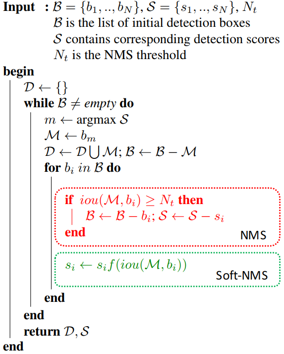
Soft NMS 算法是对 NMS 算法的改进,是发表在 ICCV2017 的论文 中提出的。NMS 算法存在一个问题是可能会把一些相邻检测框框给过滤掉(即将 IOU 大于阈值的窗口的得分全部置为 0 ),从而导致目标的 recall 指标比较低。而 Soft NMS 算法会为相邻检测框设置一个衰减函数而非彻底将其分数置为零。Soft NMS 算法流程如下图所示:
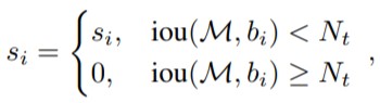
原来的 NMS 算法可以通过以下分数重置函数来描述:
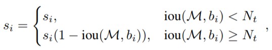
论文对 NMS 原有的分数重置函数的改进有两种形式,一种是线性加权的。设 (s_i) 为第 (i) 个 bbox 的 score, 则在应用 Soft NMS 时各个 bbox score 的计算公式如下:
另一种是高斯加权形式的,其不需要设置 iou 阈值 (N_t)。高斯惩罚系数(与上面的线性截断惩罚不同的是, 高斯惩罚会对其他所有的 bbox 作用),计算公式图如下:
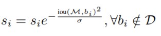
注意,这两种形式,思想都是 (M) 为当前得分最高框,(b_{i}) 为待处理框, (b_{i}) 和 (M) 的 IOU 越大,bbox 的得分 (s_{i}) 就下降的越厉害 ( (N_{t}) 为给定阈值)。Soft NMS 在每轮迭代时,先选择分数最高的预测框作为 (M),并对 (B) 中的每一个检测框 (b_i) 进行 re-score,得到新的 score,当该框的新 score 低于某设定阈值时,则立即将该框删除。
soft nms 的 python 代码如下:
def soft_nms(bboxes, Nt=0.3, sigma2=0.5, score_thresh=0.3, method=2):
    # 在 bboxes 之后添加对应的下标[0, 1, 2...], 最终 bboxes 的 shape 为 [n, 5], 前四个为坐标, 后一个为下标
    res_bboxes = deepcopy(bboxes)
    N = bboxes.shape[0]  # 总的 box 的数量
    indexes = np.array([np.arange(N)])  # 下标: 0, 1, 2, ..., n-1
    bboxes = np.concatenate((bboxes, indexes.T), axis=1)  # concatenate 之后, bboxes 的操作不会对外部变量产生影响

    # 计算每个 box 的面积
    x1 = bboxes[:, 0]
    y1 = bboxes[:, 1]
    x2 = bboxes[:, 2]
    y2 = bboxes[:, 3]
    scores = bboxes[:, 4]
    areas = (x2 - x1 + 1) * (y2 - y1 + 1)

    for i in range(N):
        # 找出 i 后面的最大 score 及其下标
        pos = i + 1
        if i != N - 1:
            maxscore = np.max(scores[pos:], axis=0)
            maxpos = np.argmax(scores[pos:], axis=0)
        else:
            maxscore = scores[-1]
            maxpos = 0

        # 如果当前 i 的得分小于后面的最大 score, 则与之交换, 确保 i 上的 score 最大
        if scores[i] < maxscore:
            bboxes[[i, maxpos + i + 1]] = bboxes[[maxpos + i + 1, i]]
            scores[[i, maxpos + i + 1]] = scores[[maxpos + i + 1, i]]
            areas[[i, maxpos + i + 1]] = areas[[maxpos + i + 1, i]]

        # IoU calculate
        xx1 = np.maximum(bboxes[i, 0], bboxes[pos:, 0])
        yy1 = np.maximum(bboxes[i, 1], bboxes[pos:, 1])
        xx2 = np.minimum(bboxes[i, 2], bboxes[pos:, 2])
        yy2 = np.minimum(bboxes[i, 3], bboxes[pos:, 3])
        w = np.maximum(0.0, xx2 - xx1 + 1)
        h = np.maximum(0.0, yy2 - yy1 + 1)
        intersection = w * h
        iou = intersection / (areas[i] + areas[pos:] - intersection)

        # Three methods: 1.linear 2.gaussian 3.original NMS
        if method == 1:  # linear
            weight = np.ones(iou.shape)
            weight[iou > Nt] = weight[iou > Nt] - iou[iou > Nt]
        elif method == 2:  # gaussian
            weight = np.exp(-(iou * iou) / sigma2)
        else:  # original NMS
            weight = np.ones(iou.shape)
            weight[iou > Nt] = 0

        scores[pos:] = weight * scores[pos:]

    # select the boxes and keep the corresponding indexes
    inds = bboxes[:, 5][scores > score_thresh]
    keep = inds.astype(int)

    return res_bboxes[keep]
六,目标检测的不平衡问题
论文 Imbalance Problems in Object Detection 给出了详细的综述。这篇论文主要是系统的分析了目标检测中的不平衡问题,并按照问题进行分类,提出了四类不平衡,并对每个问题现有的解决方案批判性的提出了观点,且给出了一个实时跟踪最新的不平衡问题研究的网页。
6.1,介绍
文章指出当有关输入属性的分布影响性能时,就会出现与输入属性相关的不平衡问题。论文将不平衡问题归为四类:
Class imbalance: 类别不平衡。不同类别的输入边界框的数量不同,包括前景/背景和前景/前景类别的不平衡,RPN和Focal Loss就是解决这类问题。Scale imbalance: 尺度不平衡,主要是目标边界框的尺度不平衡引起的,也包括将物体分配至feature pyramid时的不平衡。典型如FPN就是解决物体多尺度问题的。Spatial imbalance: 空间不平衡。包括不同样本对回归损失贡献的不平衡,IoU分布的不平衡,和目标分布位置的不平衡。Objective imbalance:不同任务(分类、回归)对总损失贡献的不平衡。
参考资料
- Focal Loss for Dense Object Detection
- NMS介绍
- Faster RCNN 源码解读(2) -- NMS(非极大抑制)
- nms
- Imbalance Problems in Object Detection: A Review
- 5分钟理解Focal Loss与GHM——解决样本不平衡利器
- focal loss 通俗讲解
- 损失函数|交叉熵损失函数
文章来源: 博客园
- 还没有人评论,欢迎说说您的想法!


 客服
客服


